# Assigning Objects
mass <- 47.5                        # assign 47.5 to "mass" (in kg)
age <- 122                          # assign 122 to "age"
mass <- mass * 2                    # multiply mass by 2
age <- age - 20                     # subtract 20 from age
mass_index <- mass/age              # divide mass by age
mass_sq <- mass^2 # raise to an exponent (2)1.2: Introduction to Coding
Learning Outcomes
- Students will be able to define the following terms:
- object
- assignment
- vector
- function
- data frame
- Students will be able to run code line-by-line and as code chunks from an Rmarkdown file.
- Students will be able to comment their code effectively.
- Students will be able to write code assign values to variables and use these variables to perform various operations.
- Students will be able to use help files to learn how to use functions.
- Students will be able to recall and explain how functions operate, and the basic syntax around functions (arguments, auto-completion, parentheses).
- Students will be able to differentiate different data classes in R.
- Students will learn how to create their own data structures (vectors, data frames).
Assigning Objects
Assignments are really key to almost everything we do in R. This is how we create permanence in R. Anything can be saved to an object, and we do this with the assignment operator, <-.
The short-cut for <- is Alt + - (or Option + - on a Mac)
This is simple and you’ll rarely do it in real-world scenarios.
1-Dimensional Data: Vectors
We can also assign more complex group of elements of the same type to a particular object. This is called a vector, a basic data structure in R.
# A group of mass values assigned to "mass_kg"
mass_kg <- c(3, 2, 4, 9, 7, 3, 6)

# View object
mass_kg
[1] 3 2 4 9 7 3 6# A group of animal names assigned to "animals"
animals <- c("cat", "rat", "bat")
# View object
animals[1] "cat" "rat" "bat"R does everything in vectors
Data classes
There are a few main types in R, and they behave differently.
- Numeric: numbers
- Integer (no decimals allowed)
- Double (decimals allowed — interchangeable with numeric)
- Character: letters or mixture
- Logical: True or False; T or F
- Factors: best used for data that need to be in a specific order; levels indicate the order
# Examples of different data classes

# We can view what class of data is in each of our objects if we call them

mass_kg       # numeric, integer, double
[1] 3 2 4 9 7 3 6animals # character[1] "cat" "rat" "bat"animal_size <- as.factor(c("small", "medium", "large"))
animal_size # factor puts in order [1] small medium large
Levels: large medium smalllogic <- c(T, F, F, T)
logic # logical[1] TRUE FALSE FALSE TRUEVectors have to contain elements that are all of the same class.
# Will this become an object?
# We will try putting in an integer, double, and character
vec <- c(1, 1.000, "1")
Sub-setting Vectors
Sometimes we want to pull out and work with specific values from a vector. This is called sub-setting (taking a smaller set of the original). To signify which element of the vector we’d like to pull out, we can use a square bracket and the number of the element we are interested in taking.
# Use square brackets

mass_kg[2]        # Pull out second element in mass_kg
[1] 2mass_kg[2:4] # Pull out 2nd, 3rd, and 4th elements from mass_kg[1] 2 4 9Functions
Functions are pre-written bits of codes that perform specific tasks for us. There are ones built into R (base R), but later in the course we will see that there are more specialized ones that we can equip using another function called library().
Functions are always followed by parentheses. Anything you type into the parentheses are called arguments.
# Functions

# Average the mass_kg vector from above
mass_kg_mean <- mean(mass_kg)

# View
mass_kg_mean
[1] 4.857143# Round the result in mass_kg mean
round(mass_kg_mean) [1] 5# Maybe we want to round to 2 digits past 0
round(mass_kg_mean, digits = 2) [1] 4.86To get more information about a function, use the help() function or ? name_of_function.
help(round) # or type ? helpWe can use a function called class() to figure out the data type of a vector.
# A function that tells us the class
class(mass_kg)
[1] "numeric"Challenge
Let’s practice! Write a few lines of code that do the following:
- Create a vector with numbers from 6 to 1 (6, 5, 4, 3, 2, 1)
- Assign the vector to an object named
vec - Subset
vecto include the last 3 numbers (should include 3, 2, 1) - Find the sum of the numbers (hint: use the
sum()function)
Answer: 6
# Make vector
vec <- c(6, 5, 4, 3, 2, 1)

# Check work
vec
[1] 6 5 4 3 2 1# Subset last three elements
vec <- vec[4:6]
# Check work
vec[1] 3 2 1# Sum final vector
sum(vec)[1] 6Already finished? See if you can condense your code down any further.
# Auto-generate sequence of numbers 6 to 1
vec <- seq(6, 1)

# From inside to outside:
# (1) subset last 3 elements in vector
# (2) sum the resulting vector
sum(vec[4:6])
[1] 62-Dimensional Data: Data Frames
Most of the data you will encounter is two-dimensional, i.e., it has columns and rows. Its structure resembles a spreadsheet. R is really good with these types of data.
- Rows go side-to-side
- Columns go up-and-down
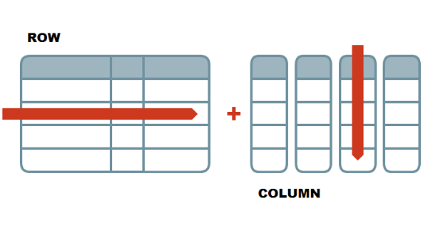
Data frames are made up of multiple vectors. Each vector becomes a column.
# Create a simple data frame
# First column is plant heights
# Next column is nitrogen T/F
plants <- data.frame(height = c(55, 17, 42, 47, 68, 39),
                     nitrogen = c("Y", "N", "N", "Y", "Y", "N"))

# View our new data frame
plants
height nitrogen
1 55 Y
2 17 N
3 42 N
4 47 Y
5 68 Y
6 39 NSub-setting Data Frames
Because data frames are two-dimensional, we can subset data in different ways. We can select specific columns, specific rows, or filter rows by values.
R always takes information for the row first, then the column.
# Sub-setting data frames

# 2-dimensional, so you need to specify row and then column as [row, column]

# plants[3] # Will not work

# Get row 4, column 1
plants[4,1]
[1] 47# Get column 2
plants[, 2][1] "Y" "N" "N" "Y" "Y" "N"Another way to pull out a single column from a data frame is with the $ operator. This can really come in handy when you know the name of the column but not the position.
# Get "height" column
plants$height
[1] 55 17 42 47 68 39Ideally, after typing $, R should give you a drop down list of all the column names that you can select from. Sometimes that doesn’t happen though, and that’s okay! You can also find column names / numbers by opening and looking through your data frame object in the Environment.
Discussion Point
This is a simple data set, but let’s come up with some questions.
Example: Height of plants treated with nitrogen vs. those not treated.
# Filter rows based on values in the nitrogen column

# Isolate plants data where nitrogen is "Y"
plants[plants$nitrogen == "Y", ]
height nitrogen
1 55 Y
4 47 Y
5 68 Y# Find the mean of plants treated with nitrogen
mean(plants[plants$nitrogen == "Y", 1])[1] 56.66667Challenge: Using help files on functions
Find the standard deviation (sd()) of the height of plants treated with nitrogen and those not treated with nitrogen. Which group has the larger standard deviation?
# Standard deviation of plants treated with nitrogen
sd(plants[plants$nitrogen == "Y", 1])
[1] 10.59874# Standard deviation of plants NOT treated with nitrogen
sd(plants[plants$nitrogen == "N", 1])[1] 13.6504Come up with a definition of standard deviation (Google is your friend!), use the help file (help() or ? function) to find out how the sd() function works, and be prepared to show the code you used.
Helpful Functions
Below are some functions that I often find very helpful when working with vectors and data frames:
str()head()andtail()length()ncol()andnrow()names()
# Structure of the object
str(plants)
'data.frame': 6 obs. of 2 variables:
$ height : num 55 17 42 47 68 39
$ nitrogen: chr "Y" "N" "N" "Y" ...# First 6 values or rows (default)
head(plants) height nitrogen
1 55 Y
2 17 N
3 42 N
4 47 Y
5 68 Y
6 39 N# First n values or rows
head(plants, n = 4) height nitrogen
1 55 Y
2 17 N
3 42 N
4 47 Y# Last n values or rows
tail(plants, n = 4) height nitrogen
3 42 N
4 47 Y
5 68 Y
6 39 N# For a dataframe, length() gives the number of columns
length(plants) [1] 2# For a column or vector, length() gives number of rows
length(plants$height) [1] 6# Number of columns
ncol(plants) [1] 2# Number of rows
nrow(plants) [1] 6# List of column or object names
names(plants) [1] "height" "nitrogen"